Creating equilibria¶

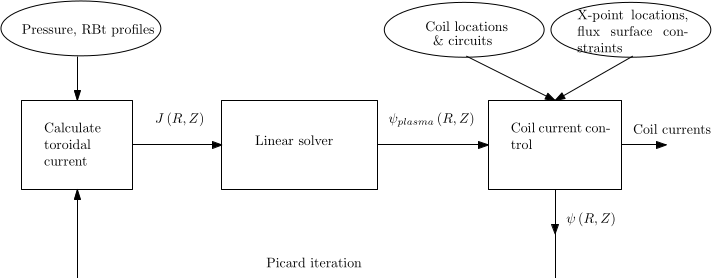
To generate a Grad-shafranov solution from scratch FreeGS needs some physical parameters:

The locations of the coils
Plasma profiles (typically pressure and a current function) used to calculate toroidal current density $J_\phi$
The desired locations of X-points, and constraints on the shape of the plasma.

and some numerical parameters:

The domain in which we want to calculate the solution
The methods to be used to solve the equations

These inputs are combined in a nonlinear Picard iteration with the main components shown in the figure below.

Main components in the Picard iteration used to solve free boundary equilibrium problem.

Tokamak coils, circuits and solenoid¶

Example 1 (01-freeboundary.py) creates a simple lower single null plasma from scratch. First import the freegs library

import freegs

then create a tokamak, which specifies the location of the coils. In this example this is done using

tokamak = freegs.machine.TestTokamak()

which creates an example machine with four poloidal field coils (two for the vertical field, and two for the radial field). To define a custom machine, first create a list of coils:

from freegs.machine import Coil

coils = [("P1L", Coil(1.0, -1.1)),
          ("P1U", Coil(1.0, 1.1)),
          ("P2L", Coil(1.75, -0.6)),
          ("P2U", Coil(1.75, 0.6))]

Each tuple in the list defines the name of the coil (e.g. "P1L"), then the corresponding object (e.g. Coil(1.0, -1.1) ). Here Coil(R, Z) specifies the R (major radius) and Z (height) location of the coil in meters.

Create a tokamak by passing the list of coils to Machine:

tokamak = freegs.machine.Machine(coils)

Coil current control¶

By default all coils can be controlled by the feedback system, but it may be that you want to fix the current in some of the coils. This can be done by turning off control and setting the current:

Coil(1.0, -1.1, control=False, current=50000.)

where the current is in Amps, and is for a coil with a single turn. Setting control=False removes the coil from feedback control.

Shaped coils¶

The ShapedCoil class models a coil with uniform current density across a specified shape (a polygon). This is done by splitting the polygon into triangles (using the ear clipping method) and then using Gaussian quadrature to integrate over each triangle (by default using 6 points per triangle). The shape of the coil should be specified as a list of (R,Z) points:

from freegs.machine import ShapedCoil

coils = [("P1L", ShapedCoil([(0.95, -1.15), (0.95, -1.05), (1.05, -1.05), (1.05, -1.15)])),
         ...]

The above would create a square coil. The number of turns and the current in the circuit can be specified:

coils = [("P1L", ShapedCoil([(0.95, -1.15), (0.95, -1.05), (1.05, -1.05), (1.05, -1.15)],
                            current = 1e3, turns=20)),
         ...]

The number of turns doesn’t affect the integration, but the total current in the coil block is set to current * turns.

Multi strand coils¶

The MultiCoil class provides a way to model a coil block with turns in specified locations. For large numbers of turns this is usually more convenient than creating multiple Coil objects. A MultiCoil can be used anywhere a Coil object would be:

from freegs.machine import MultiCoil

coils = [ ("P2", MultiCoil([0.95, 0.95, 1.05, 1.05], [1.15, 1.05, 1.05, 1.15])) ]

For coils which are wired together as pairs, mirrored in Z, the mirror=True keyword can be given. The polarity keyword then sets the relative sign of the current in the original and mirrored coil.

Coil circuits¶

Usually not all coils in a tokamak are independently powered, but several coils may be connected to the same power supply. This is handled in FreeGS using Circuit objects, which consist of several coils. For example:

from freegs.machine import Circuit

Circuit( [("P2U", Coil(0.49,  1.76), 1.0),
          ("P2L", Coil(0.49, -1.76), 1.0)] )

This creates a Circuit by passing a list of tuples. Each tuple defines the coil name, the Coil object (with R,Z location), and a current multiplier. In this case the current multiplier is 1.0 for both coils, so the same current will flow in both coils. Alternatively coils may be wired in opposite directions:

Circuit( [("P6U", Coil(1.5,  0.9), 1.0),
          ("P6L", Coil(1.5, -0.9), -1.0)] )

so the current in coil “P6L” is in the opposite direction, but same magnitude, as the current in coil “P6U”.

As with coils, circuits by default are controlled by the feedback system, and can be fixed by setting control=False and specifying a current.

Solenoid¶

Tokamaks typically operate with Ohmic current drive using a central solenoid. Flux leakage from this solenoid can modify the equilibrum, particularly the locations of the strike points. Solenoids are represented in FreeGS by a set of poiloidal coils:

from freegs.machine import Solenoid

solenoid = Solenoid(0.15, -1.4, 1.4, 100)

which defines the radius of the solenoid in meters (0.15m here), the lower and upper limits in Z (vertical position, here $\pm$ 1.4 m), and the number of poloidal coils to be used. These poloidal coils will be equally spaced between the lower and upper Z limits.

As with Coil and Circuit, solenoids can be removed from feedback control by setting control=False and specifying a fixed current.

Mega-Amp Spherical Tokamak¶

As an example, the definition of the Mega-Amp Spherical Tokamak (MAST) coilset is given in the freegs.machine.MAST_sym() function:

coils = [("P2", Circuit( [("P2U", Coil(0.49,  1.76), 1.0),
                           ("P2L", Coil(0.49, -1.76),1.0)] ))
         ,("P3", Circuit( [("P3U", Coil(1.1,  1.1), 1.0),
                           ("P3L", Coil(1.1, -1.1), 1.0)] ))
         ,("P4", Circuit( [("P4U", Coil(1.51,  1.095), 1.0),
                           ("P4L", Coil(1.51, -1.095), 1.0)] ))
         ,("P5", Circuit( [("P5U", Coil(1.66,  0.52), 1.0),
                           ("P5L", Coil(1.66, -0.52), 1.0)] ))
         ,("P6", Circuit( [("P6U", Coil(1.5,  0.9), 1.0),
                            ("P6L", Coil(1.5, -0.9), -1.0)] ))
         ,("P1", Solenoid(0.15, -1.45, 1.45, 100))
        ]

 tokamak = freegs.machine.Machine(coils)

This uses circuits “P2” to “P5” connecting pairs of upper and lower coils in series. Circuit “P6” has its coils connected in opposite directions, so is used for vertical position control. Finally “P1” is the central solenoid. Here all circuits and solenoid are under position feedback control.

Machine walls (limiters)¶

The internal walls of the machine are specified by a polygon in R-Z i.e. an ordered list of (R,Z) points which form a closed boundary. These are stored in a Wall object:

from freegs.machine import Wall

wall = Wall([ 0.75, 0.75,  1.5,  1.8,   1.8,   1.5],   # R
            [-0.85, 0.85, 0.85, 0.25, -0.25, -0.85])   # Z

The wall can then be specified when creating a machine:

tokamak = freegs.machine.Machine(coils, wall)

or an existing machine can be modified:

tokamak.wall = wall

Note that the location of these walls does not currently affect the equilibrium, but is used by some diagnostics, and is written to output files such as EQDSK format.

Sensors¶

Rogowski (Rog), Poloidal Field (BP), and Flux Loop (FL) sensors can be added to the machine.

Each individual sensor inherits from the Sensor class, which have inputs as follows:

class Sensor:
    def __init__(self, R, Z, name=None, weight=1, status=True, measurement=None):

R and Z take the input for the position of the sensors.

The weight is an attribute that is useful to consider with reconstruction on real data, can be thought of as the inverse of the sensor measurement uncertainty. Will discuss more in future chapters.

The status of a sensor determines whether it is turned on or not, and therefore whether it will take a measurement when takeMeasurement method of machine is called.

A list of sensors can be specified when creating a machine:

tokamak = freegs.machine.Machine(coils, wall, sensors)

Rogowski Sensors¶

Rog sensors measure the total current within their shape. The R-Z input is the same as the Wall class, taking an ordered list of (R,Z) points which form a closed boundary.

BP Sensors¶

BP sensors measure the poloidal field at a given angle. They are effectively ‘point’ sensors so single values for R and Z are given, aswell as a value for theta (angle of measurement)

FL Sensors¶

FL sensors measure the flux at an R,Z position. They are also point sensors, so need a single value for R and Z input.

Adding each one of these sensors to a machine when creating can be done as follows:

sensors = [RogowskiSensor(R = [ 0.75, 0.75,  1.5,  1.8,   1.8,   1.5],
                          Z = [-0.85, 0.85, 0.85, 0.25, -0.25, -0.85]),
            PoloidalFieldSensor(R = 0.75, Z = 1, theta = 0.9),
            FluxLoopSensor(R = 1.8, Z = 0.2)]

tokamak = Machine(coils, wall, sensors)

Equilibrium and plasma domain¶

Having created a tokamak, an Equilibrium object can be created. This represents the plasma solution, and contains the tokamak with the coil currents.

eq = freegs.Equilibrium(tokamak=tokamak,
                     Rmin=0.1, Rmax=2.0,    # Radial domain
                     Zmin=-1.0, Zmax=1.0,   # Height range
                     nx=65, ny=65)          # Number of grid points

In addition to the tokamak Machine object, this must be given the range of major radius R and height Z (in meters), along with the radial (x) and vertical (y) resolution. This resolution must be greater than 3, and is typically a power of 2 + 1 ( $2^n+1$ ) for efficiency, but does not need to be.

Boundaries¶

The boundary conditions to be applied are set when an Equilibrium object is created, since this forms part of the specification of the domain. By default a free boundary condition is set, using an accurate but inefficient method which integrates the Greens function over the domain. For every point $\mathbf{\left(R_b,Z_b\right)}$ on the boundary the flux is calculated using

$\psi\left(R_b,Z_b\right) = \iint G(R, Z; R_b, Z_b) J_\phi\left(R,Z\right) dRdZ$

where $G$ is the Greens function.

An alternative method, which scales much better to large grid sizes, is von Hagenow’s method. To use this, specify the freeBoundaryHagenow boundary function:

eq = freegs.Equilibrium(tokamak=tokamak,
                     Rmin=0.1, Rmax=2.0,    # Radial domain
                     Zmin=-1.0, Zmax=1.0,   # Height range
                     nx=65, ny=65,          # Number of grid points
                     boundary=freegs.boundary.freeBoundaryHagenow)

Alternatively for simple tests the fixedBoundary function sets the poloidal flux to zero on the computational boundary.

Conducting walls¶

To specify a conducting wall on which the poloidal flux is fixed, so that there is a skin current on the wall, a series of coils can be used. The current in each coil is set using the feedback controller, to satisfy a fixed poloidal flux constraint.

For the full example code, see (and try running) 09-metal-wall.py.

First create an array of R,Z locations, here called Rwalls and Zwalls. For example a circular wall:

R0 = 1.0     # Middle of the circle
rwall = 0.5  # Radius of the circular wall

npoints = 200 # Number of points on the wall

# Poloidal angles
thetas = np.linspace(0, 2*np.pi, npoints, endpoint=False)

# Points on the wall
Rwalls = R0 + rwall * np.cos(thetas)
Zwalls = rwall * np.sin(thetas)

Then create a set of coils, one at each of these locations:

coils = [ ("wall_"+str(theta),    # Label
           freegs.machine.Coil(R, Z)) # Coil at (R,Z)
          for theta, R, Z in zip(thetas, Rwalls, Zwalls) ]

The label doesn’t have to be unique , but having unique names makes referring to them later easier. The tokamak can then be created:

tokamak = freegs.machine.Machine(coils)

The next part is to control the currents in the coils using fixed poloidal flux constraints:

psivals = [ (R, Z, 0.0) for R, Z in zip(Rwalls, Zwalls) ]

This is a list of (R, Z, value) tuples, which specify that the poloidal flux should be fixed to zero (in this case) at the given (R,Z) location. The control system is then created:

constrain = freegs.control.constrain(psivals=psivals)

The final modification to the usual solve is that we can specify a poloidal flux for the plasma boundary:

freegs.solve(eq,          # The equilibrium to adjust
           profiles,    # The toroidal current profile function
           constrain,   # Constraint function to set coil currents
           psi_bndry=0.0)  # Because no X-points, specify the separatrix psi

If psi_bndry is set then this overrides the usual process, which uses the innermost X-point to set the plasma boundary psi. In this case there are some X-points between coils, but its more reliable to set the boundary like this.

Plasma profiles¶

The plasma profiles, such as pressure or safety factor, are used to determine the toroidal current $J_\phi$ :

$J_\phi\left(R,Z\right) = R\frac{\partial p\left(\psi\right)}{\partial \psi} + \frac{f\left(\psi\right)}{R\mu_0}\frac{\partial f\left(\psi\right)}{\partial \psi}$

where the flux function $p\left(\psi\right)$ is the plasma pressure (in Pascals), and $f\left(\psi\right) = RB_\phi$ is the poloidal current function. Classes and functions to handle these profiles are in freegs.jtor

Constrain pressure and current¶

One of the most intuitive methods is to fix the shape of the plasma profiles, and adjust them to fix the pressure on the magnetic axis and total plasma current. To do this, create a ConstrainPaxisIp profile object:

profiles = freegs.jtor.ConstrainPaxisIp(1e4, # Pressure on axis [Pa]
                                        1e6, # Plasma current [Amps]
                                        1.0) # Vacuum f=R*Bt

This sets the toroidal current to:

$J_\phi = L \left[\beta_0 R + \left(1-\beta_0\right)/R\right] \left(1-\psi_n^{\alpha_m}\right)^{\alpha_n}$

where $\psi_n$ is the normalised poloidal flux, 0 on the magnetic axis and 1 on the plasma boundary/separatrix. The constants which determine the profile shapes are $\alpha_m = 1$ and $\alpha_n = 2$ . These can be changed by specifying in the initialisation of ConstrainPaxisIp.

The values of $L$ and $\beta_0$ are determined from the constraints: The pressure on axis is given by integrating the pressure gradient flux function

$p_{axis} = - L \beta_0 R \int_{axis}^{boundary}\left(1-\psi_n^{\alpha_m}\right)^{\alpha_n} d\psi$

The total toroidal plasma current is calculated by integrating the toroidal current function over the 2D domain:

$I_p = L\beta_0 \iint R \left(1-\psi_n^{\alpha_m}\right)^{\alpha_n} dR dZ + L\left(1-\beta_0\right)\iint \frac{1}{R} \left(1-\psi_n^{\alpha_m}\right)^{\alpha_n} dR dZ$

The integrals in these two constraints are done numerically, and then rearranged to get $L$ and $\beta_0$ .

Constrain poloidal beta and current¶

This is a variation which replaces the constraint on pressure with a constraint on poloidal beta:

$\beta_p = \frac{8\pi}{\mu_0} \frac{1}{I_p^2}\iint p\left(\psi\right) dRdZ$

This is the method used in Y.M.Jeon 2015, on which the profile choices here are based.

profiles = freegs.jtor.ConstrainBetapIp(0.5, # Poloidal beta
                                        1e6, # Plasma current [Amps]
                                        1.0) # Vacuum f=R*Bt

By integrating over the plasma domain and combining the constraints on poloidal beta and plasma current, the values of $L$ and $\beta_0$ are found.

Feedback and shape control¶

To determine the currents in the coils, the shape and position of the plasma needs to be constrained. In addition, diverted tokamak plasmas are inherently vertically unstable, and need vertical position feedback to maintain a stationary equilibrium. If vertical position is not constrained, then free boundary equilibrium solvers can also become vertically unstable. A typical symptom is that each nonlinear iteration of the solver results in a slightly shifted or smaller plasma, until the plasma hits the boundary, disappears, or forms unphysical shapes causing the solver to fail.

Currently the following kinds of constraints are implemented:

X-point constraints adjust the coil currents so that X-points (nulls in the poloidal field) are formed at the locations requested.
Isoflux constraints adjust the coil currents so that the two locations specified have the same poloidal flux. This usually means they are on the same flux surface, but not necessarily.
Psi value constraints, which adjust the coil currents so that given locations have the specified flux.

As an example, the following code creates a feedback control with two X-point constraints and one isoflux constraint:

xpoints = [(1.1, -0.6),   # (R,Z) locations of X-points
           (1.1, 0.8)]

isoflux = [(1.1,-0.6, 1.1,0.6)] # (R1,Z1, R2,Z2) pairs

constrain = freegs.control.constrain(xpoints=xpoints, isoflux=isoflux)

The control system determines the currents in the coils which are under feedback control, using the given constraints. There may be more unknown coil currents than constraints, or more constraints than coil currents. There may therefore be either no solution or many solutions to the constraint problem. Here Tikhonov regularisation is used to produce a unique solution and penalise large coil currents.

Solving¶

To solve the Grad-Shafranov equation to find the free boundary solution, call freegs.solve:

freegs.solve(eq,          # The equilibrium to adjust
             profiles,    # The toroidal current profile
             constrain)   # Feedback control

This call modifies the input equilibrium (eq), finding a solution based on the given plasma profiles and shape control.

The Grad-Shafranov equation is nonlinear, and is solved using Picard iteration. This consists of calculating the toroidal current $J_\phi$ given the poloidal flux $\psi\left(R,Z\right)$ , then solving a linear elliptic equation to calculate the poloidal flux from the toroidal current. This loop is repeated until a given relative tolerance is achieved:

$\texttt{rtol} = \frac{\textrm{change in psi}}{ \max(\psi) - \min(\psi)}$

To see how the solution is evolving at each nonlinear iteration, for example to diagnose a failing solve, set show=True in the solve call. To add a delay between iterations set pause=2.0 using the desired delay in seconds.

Inner linear solver¶

To calculate the poloidal flux given the toroidal current, an elliptic equation must be solved. To do this a multigrid scheme is implemented, which uses Jacobi iterations combined with SciPy’s sparse matrix direct solvers at the coarsest level.

By default the multigrid is not used, and SciPy’s direct solver is used for the full grid. This is because for typical grid resolutions (65 by 65) this has been found to be fastest. The multigrid method will however scale efficiently to larger grid sizes.

The easiest way to adjust the solver settings is to call the Equilibrium method setSolverVcycle. For example

eq.setSolverVcycle(nlevels = 4, ncycle = 2, niter = 10, direct=True)

This specifies that four levels of grid resolution should be used, including the original. In order to be able to coarsen (restrict) a grid, the number of points in both R and Z dimensions should be an odd number. This is one reason why grid sizes are usually $2^n + 1$ ; it allows the maximum number of multigrid levels.

The number of V-cycles (finest -> coarsest -> finest) is given by ncycle. At each level of refinement the number of Jacobi iterations to perform before restriction and again after interpolation is niter. At the coarsest level of refinement the default is to use a direct (sparse) solver.

Some experimentation is needed to find the optimium settings for a given problem.