Diagnostics#
Once an equilibrium has been generated (see Creating equilibria)
there are routines for diagnosing and calculating derived quantities.
Here the Equilibrium object is assumed to be called eq and the
Tokamak object called tokamak.
Safety factor, q#
The safety factor \(q\) at a given normalised poloidal flux
\(\psi_{norm}\) (0 on the magnetic axis, 1 at the separatrix) can
be calculated using the q(psinorm) function:
eq.q(0.9) # safety factor at psi_norm = 0.9
Note that calculating \(q\) on either the magnetic axis or separatrix is problematic, so values calculated at \(\psi_{norm}=0\) and \(\psi_{norm}=1\) are likely to be inaccurate.
This function can be used to print the safety factor on a set of flux surfaces:
print("\nSafety factor:\n\tpsi \t q")
for psi in [0.01, 0.9, 0.95]:
  print("\t{:.2f}\t{:.2f}".format(psi, eq.q(psi)))
If no value is given for the normalised psi, then a uniform array of values between 0 and 1 is generated (not including the end points). In this case both the values of normalised psi and the values of q are returned:
psinorm, q = eq.q()
which can be used to make a plot of the safety factor:
import matplotlib.pyplot as plt

plt.plot(*eq.q())
plt.xlabel(r"Normalised $\psi$")
plt.ylabel(r"Safety factor $q$")
plt.show()
Poloidal beta#
The poloidal beta \(\beta_p\) is given by:
betap = eq.poloidalBeta()
This is calculated using the expression
i.e. the same calculation as is done in the poloidal beta constraint Constrain poloidal beta and current.
Plasma pressure#
The pressure at a specified normalised psi is:
p = eq.pressure(0.0) # Pressure on axis
Separatrix location#
A set of points on the separatrix, measured in meters:
RZ = eq.separatrix()

R = RZ[:,0]
Z = RZ[:,1]

import matplotlib.pyplot as plt
plt.plot(R,Z)
Currents in the coils#
The coil objects can be accessed and their currents queried. The current in a coil named “P1L” is given by:
eq.tokamak["P1L"].current
The currents in all coils can be printed using:
tokamak.printCurrents()
which is the same as:
for label, coil in eq.tokamak.coils:
  print(label + " : " + str(coil))
Forces on the coils#
The forces on all poloidal field coils can be calculated and returned as a dictionary:
eq.getForces()
or formatted and printed:
eq.printForces()
These forces on the poloidal coils are due to a combination of:
The magnetic fields due to other coils
The magnetic field of the plasma
A self (hoop) force due to the coil’s own current
The self force is the most difficult to calculate, since the force depends on the cross-section of the coil. The formula used is from David A. Garren and James Chen (1998). For a circular current loop of radius \(R\) and minor radius \(a\), the outward force per unit length is:
where \(\xi_i\) is a constant which depends on the internal current distribution. For a constant, uniform current \(\xi_i = 1/2\); for a rapidly varying surface current \(\xi_i = 0\).
For the purposes of calculating this force the cross-section is assumed to be circular. The area can be set to a fixed value:
tokamak["P1L"].area = 0.01 # Area in m^2
where here “P1L” is the label of the coil. The default is to calculate the area using a limit on the maximum current density. A typical value chosen here for Nb3Sn superconductor is \(3.5\times 10^9 A/m^2\), taken from Kalsi (1986) .
This can be changed e.g:
from freegs import machine

tokamak["P1L"].area = machine.AreaCurrentLimit(1e9)
would set the current limit for coil “P1L” to 1e9 Amps per square meter.
Sensor Measurements#
For a machine populated with sensors, to run the get_Measure(equilibrium)
method of each sensor, tokamak.takeMeasurments(equilibrium) is used. The measurement
atrribute of each sensor is then updated with the measured values. If no equilibrium object
is passed, then the sensors will find the coil contribution (and in a future update, vessel current contribution)
to each of the measurements.
To measure and print the values, the following method is used:
from freegs import machine
tokamak = machine.TestTokamakSensor()

tokamak.printMeasurements(equilibrium)
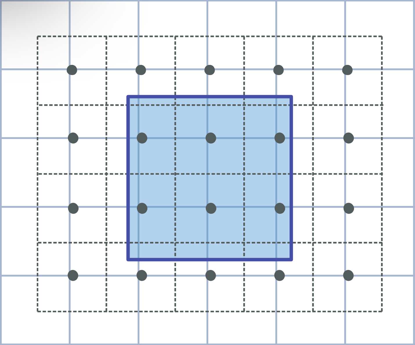
The Rogowski Coils uses a nearest neighbour interpolation method. The following diagram illustrates this. The points correspond to each grid point on the equilibrium grid. A shapely square object is created, centered around the point. The sensor calculates the intersection area of each square with the rog and multiplies it by the value of the current density at that point.
Both the BP and FL sensors use pre specified methods using interpolation in the machine and equilibrium classes.
Field line connection length#
Example: 10-mastu-connection.py. Requires the file mast-upgrade.geqdsk
which is created by running 08-mast-upgrade.py.
To calculate the distance along magnetic field lines from the outboard midplane
to the walls in an equilibrium eq, the simplest way is:
from freegs import fieldtracer
forward, backward = fieldtracer.traceFieldLines(eq)
To also plot the field lines on top of the equilibrium:
axis = eq.plot(show=False)
forward, backward = fieldtracer.traceFieldLines(eq, axis=axis)
plt.show()
This will display the poloidal cross-section of the plasma, and plot field lines traced in both directions along the magnetic field from the outboard midplane.
To plot the distances along the magnetic field from midplane to target as a function of the starting radius:
plt.plot(forward.R[0,:], forward.length[-1,:], label="Forward")
plt.plot(backward.R[0,:], backward.length[-1,:], label="Backward")
plt.legend()
plt.xlabel("Starting major radius [m]")
plt.ylabel("Parallel connection length [m]")

plt.show()
Here forward.R and forward.length are 2D arrays, where the first index
is the point along the magnetic field (0 = start, -1 = end), and the second
index is the field line number. There is also forward.Z with the height in meters.
The output can be customised by passing keywords to traceFieldLines:
solwidth sets the width of the starting region at the outboard midplane;
nlines is the number of field lines to follow in each direction;
nturns the number of times around the torus to follow the field;
npoints is the number of points along each field line.
For more control over which field lines are followed, the FieldTracer class
does the actual field line following:
from freegs import fieldtracer
import numpy as np

tracer = fieldtracer.FieldTracer(eq)

result = tracer.follow([1.35], [0.0], np.linspace(0.0, 2*np.pi, 20))
This follows a magnetic field in the direction of B, starting at \(R=1.35m\), \(Z=0\), outputting positions at 20 toroidal angles between 0 and 2pi i.e. one toroidal turn. The R and Z starting locations should be an array or list with the same shape.
The result is an array: The first index is the angle (size 20 here), and the
last index has size 3 (R, Z, length). Between the first and last indices the
result has the same shape as the R and Z starting positions. In the above code
result has size (20, 1, 3). To plot the field line on top of the
equilibrium:
import matplotlib.pyplot as plt

eq.plot(show=False)
plt.plot(result[:,0,0], result[:,0,1])
plt.show()
The direction to follow along the field can be reversed by passing
backward=True keyword to tracer.follow.